QC3｜正規分布と二項分布、確率の求め方を例題で解説　QC3 | Normal & Binomial Distributions: How to Calculate Probabilities with Examples

QC3の「統計的方法の基礎」で、多くの受験者がつまずくのが正規分布と二項分布です。正規分布表の読み方がわからない、標準化の計算で手が止まる、二項分布との違いがあいまい——こうした悩みを抱えていませんか？

One of the topics that trips up many QC3 candidates in the “Fundamentals of Statistical Methods” section is normal distribution and binomial distribution. Do you find yourself unsure how to read a normal distribution table, stuck on standardization calculations, or unclear on the difference between the two distributions?

この記事では、正規分布と二項分布の基本的な考え方から、標準化の計算手順、正規分布表の具体的な使い方、そして試験で頻出の確率の求め方パターンまでを、例題を交えてわかりやすく解説します。

This article explains everything from the basic concepts of normal and binomial distributions, to the step-by-step procedure for standardization, practical guidance on using the normal distribution table, and the most frequently tested patterns for calculating probabilities — all with worked examples.

QC3では、正規分布の出題頻度が非常に高く、ここを確実に得点できるかどうかが合否を分けるポイントになります。数学や統計に苦手意識がある方でも理解できるように、計算の一つひとつを丁寧に追っていきますので、安心して読み進めてください。

Normal distribution questions appear with very high frequency in QC3, and whether you can score reliably on them is often what separates those who pass from those who do not. Each calculation is explained carefully so that even those who find mathematics or statistics daunting can follow along with confidence.

正規分布とは？｜計量値の分布を理解しよう　What Is Normal Distribution? | Understanding the Distribution of Measured Values

品質管理の現場では、「不良品がどれくらいの割合で出るのか」をあらかじめ予測できると、対策が立てやすくなります。そのために必要なのが「確率と分布」の考え方です。

In quality management, being able to predict in advance what proportion of products will be defective makes it much easier to take preventive action. The key to doing this lies in understanding the concepts of probability and distribution.

確率とは、ある出来事がどれくらい起こりやすいかを表す数字です。たとえば、サイコロを振って1が出る確率は6分の1（約16.7%）です。これと同じように、工場で作った製品の重さや長さについても、「ある値になる確率はどれくらいか」を考えることができます。

Probability is a number that expresses how likely a particular event is to occur. For example, the probability of rolling a 1 on a die is one in six (approximately 16.7%). In the same way, it is possible to ask “what is the probability of a product weighing or measuring a particular value?” for items produced in a factory.

たとえば、同じ工場で同じペットボトル飲料を作っても、内容量はぴったり500mlにはなりません。499mlのときもあれば、501mlのときもあります。このように、データには必ずばらつきがあります。

For example, even when the same factory produces the same bottled beverage, the contents will never be exactly 500 ml every time — sometimes it will be 499 ml, sometimes 501 ml. All data, without exception, contains variation.

しかし、このばらつき方はデタラメではありません。実は一定のルールに従っていて、「どのような値が、どれくらいの確率で現れるか」はあらかじめ決まっています。このばらつき方のルールのことを分布（確率分布）といいます。

However, this variation is not random. It follows consistent rules, and “which values appear and how often” is determined in advance. This set of rules governing how values are spread is called a distribution (probability distribution).

QC3で出題される分布は、正規分布と二項分布の2つです。正規分布は計量値（長さや重さなど、連続した値）の分布を表し、二項分布は計数値（不適合品数や人数など、1つ、2つと数えられる値）の分布を表します。

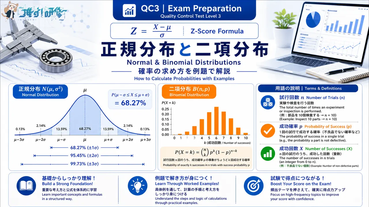
The two distributions tested in QC3 are normal distribution and binomial distribution. Normal distribution describes the distribution of measured values (continuous values such as length and weight), while binomial distribution describes the distribution of counted values (discrete values such as the number of nonconforming items or the number of people).

正規分布の形と特徴　The Shape and Characteristics of Normal Distribution

正規分布の形には、次のような特徴があります。

The shape of normal distribution has the following characteristics.

• 左右対称の釣鐘型（お寺の鐘を横から見たような形）
  Symmetrical bell shape (resembling a temple bell viewed from the side)
• 山の頂上は必ず1つだけ
  Exactly one peak
• 左右が非対称になったり、山が2つになることはない
  It is always symmetric about the mean, and never has two peaks

イメージとしては、クラス全員のテストの点数をグラフにしたときの形を思い浮かべてください。平均点のあたりに一番多くの人が集まり、そこから離れるほど人数が少なくなっていく、あの山型のグラフが正規分布です。

Picture the shape you would get if you plotted the test scores of an entire class on a graph. The largest number of students clusters around the average, with fewer and fewer students as you move away from the centre — that bell-shaped curve is normal distribution.

山の高さや裾の広がり方は、データによって変わります。ばらつきが小さいデータなら細長い山になり、ばらつきが大きいデータなら横に広がった山になります。

The height of the peak and the spread of the tails vary depending on the data. Data with small variation produces a tall, narrow peak, while data with large variation produces a wide, flatter shape.

正規分布のパラメータ：平均μと分散σ²　Parameters of Normal Distribution: Mean μ and Variance σ²

では、正規分布の山の形は何によって決まるのでしょうか。それが、平均μ（ミュー）と分散σ²（シグマの二乗）という2つのパラメータです。パラメータとは、分布の形を決める要素のことです。

So what determines the shape of the normal distribution curve? The answer is two parameters: the mean μ (mu) and the variance σ² (sigma squared). Parameters are the elements that define the shape of a distribution.

正規分布はN(μ, σ²)と表します。試験の問題文では、「○○のデータは正規分布N(μ, σ²)に従う」という書かれ方をします。

Normal distribution is written as N(μ, σ²). In exam questions, you will typically see phrasing such as “the data for ○○ follows a normal distribution N(μ, σ²).”

平均μは「山の中心がどこにあるか」を表し、分散σ²は「山がどれくらい横に広がっているか」を表します。平均μが山の位置を決め、分散σ²が山の形を決める——このイメージを持っておくと理解しやすくなります。

The mean μ indicates where the centre of the peak sits, while the variance σ² indicates how widely the curve spreads horizontally. Think of it this way: μ determines the position of the peak, and σ² determines its shape.

ここでいう平均μと分散σ²は、母集団（調べたい対象の全体）の平均と分散のことで、正確にはそれぞれ母平均、母分散といいます。母分散σ²は母標準偏差σの二乗なので、正規分布のパラメータは「母平均と母標準偏差」と書かれることもあります。

The mean μ and variance σ² referred to here are the mean and variance of the population (the entire group being studied), more precisely called the population mean and population variance. Since the population variance σ² is the square of the population standard deviation σ, the parameters of normal distribution are sometimes written as “population mean and population standard deviation.”

なお、平均値x̄、不偏分散V、標準偏差sは、母集団の一部を取り出して計算した値です。母集団全体のパラメータとは意味が異なるため、記号も違うものを使います。この違いは試験でもよく問われるポイントです。

Note that the sample mean x̄, sample variance V (unbiased estimator), and sample standard deviation s are values calculated from a subset of the population. Because they differ in meaning from the parameters of the full population, different symbols are used. This distinction is a frequently tested point in the exam.

標準正規分布 N(0, 1²) とは　What Is the Standard Normal Distribution N(0, 1²)?

正規分布の中でも特別なものがあります。平均μが0、分散σ²が1の正規分布N(0, 1²)を、標準正規分布といいます。

Among all normal distributions, there is one of special importance. The normal distribution N(0, 1²), with a mean μ of 0 and a variance σ² of 1, is called the standard normal distribution.

なぜ特別かというと、正規分布表はこの標準正規分布N(0, 1²)をもとに作られているからです。つまり、どんな正規分布でも、標準正規分布に変換しさえすれば、正規分布表を使って確率を求めることができるのです。

The reason it is special is that the normal distribution table is built on this standard normal distribution N(0, 1²). In other words, any normal distribution can be converted into the standard normal distribution, after which the normal distribution table (standard normal table / Z-table) can be used to find probabilities.

この変換作業のことを「標準化（規準化）」といいます。次のセクションで、標準化の具体的な計算方法を見ていきましょう。

This conversion process is called standardization (or normalization). In the next section, we will look at the specific calculation procedure for standardization.

標準化（Z変換）の計算方法　How to Calculate Standardization (Z-Transformation)

正規分布N(μ, σ²)を標準正規分布N(0, 1²)に変換する作業が「標準化」です。やっていることは、「今あるデータを、平均0・分散1の世界に置き換える」ことです。標準化を行えば、どんな正規分布でも、1つの共通の表（正規分布表）を使って確率が求められるようになります。

Standardization is the process of converting a normal distribution N(μ, σ²) into the standard normal distribution N(0, 1²). In essence, it means “re-expressing your data in a world where the mean is 0 and the variance is 1.” Once standardization is performed, a single shared table — the normal distribution table — can be used to find probabilities for any normal distribution.

標準化の式：Z =（x − μ）/ σ　The Standardization Formula: Z = (x − μ) / σ

標準化の式は次の通りです。

The standardization formula is as follows.

Z = (x − μ) / σ

それぞれの意味を確認しましょう。

Let us confirm what each element means.

• x：確率を求めたい値（たとえば「○g以下になる確率」の○にあたる数字）
  The value for which you want to find a probability (e.g., the number in “the probability of being ○g or less”)
• μ：平均（正規分布の中心の値）
  The mean (the central value of the normal distribution)
• σ：標準偏差（ばらつきの大きさ）
  The standard deviation (the size of the variation)
• Z：標準化された値（これを使って正規分布表を読む）
  The standardized value (used to read the normal distribution table)

この式が意味しているのは、「xが平均μからどれだけ離れているかを、標準偏差σの何個分かで表す」ということです。

What this formula expresses is “how far x is from the mean μ, measured in units of the standard deviation σ.”

この式は必ず覚えてください。試験では、問題文で与えられたμ、σ、xの値をこの式にあてはめて計算するだけで解ける問題が多く出題されます。

Make sure to memorize this formula. Many exam questions can be solved simply by substituting the values of μ, σ, and x given in the question into this formula.

標準化の計算例　A Worked Example of Standardization

具体例で確認しましょう。

Let us confirm this with a concrete example.

ある工場で生産しているボルトの長さは、平均μ = 50mm、標準偏差σ = 2mmの正規分布に従っています。このとき、「長さが46mm以下になる確率」を求めるために標準化を行います。

The length of bolts produced at a certain factory follows a normal distribution with a mean μ = 50mm and a standard deviation σ = 2mm. We will now perform standardization in order to find “the probability that the length is 46mm or less.”

Z = (x − μ) / σ = (46 − 50) / 2 = −2.0

計算結果のZ = −2.0は、「46mmという値は、平均50mmから標準偏差2mmの2個分だけ下（左）にある」ということを意味しています。

The result Z = −2.0 means that “the value of 46mm is 2 standard deviations (of 2mm each) below (to the left of) the mean of 50mm.”

Zは標準正規分布N(0, 1²)に従います。このZの値を使って、次のステップで正規分布表から確率を読み取ります。

Z follows the standard normal distribution N(0, 1²). Using this value of Z, the next step is to read the probability from the normal distribution table.

正規分布表の使い方｜K_PからPを求める　How to Use the Normal Distribution Table | Finding P from K_P

正規分布に従うデータから確率を求める問題は、QC3で非常によく出題されます。ここでは、正規分布表の読み方と、確率を求めるための3つのパターンを解説します。

Questions that require finding probabilities from normally distributed data appear very frequently in QC3. This section explains how to read the normal distribution table and covers three patterns for calculating probabilities.

まず、この記事で使用する正規分布表を掲載します。試験では問題用紙の最後に正規分布表が載っているので覚える必要はありませんが、読み方を練習するために活用してください。

The normal distribution table used in this article is provided below. Since the table is printed at the end of the exam paper, you do not need to memorize it — but use it to practice reading the values.

正規分布表（I）K_PからPを求める表　Normal Distribution Table (I): Finding P from K_P

標準化で求めたZの絶対値をK_Pとして、対応する確率Pを読み取る表です。

This table is used to look up the corresponding probability P for a given value of K_P, which is the absolute value of the standardized Z.

KP	*=0	1	2	3	4	5	6	7	8	9
0.0*	.5000	.4960	.4920	.4880	.4840	.4801	.4761	.4721	.4681	.4641
0.1*	.4602	.4562	.4522	.4483	.4443	.4404	.4364	.4325	.4286	.4247
0.2*	.4207	.4168	.4129	.4090	.4052	.4013	.3974	.3936	.3897	.3859
0.3*	.3821	.3783	.3745	.3707	.3669	.3632	.3594	.3557	.3520	.3483
0.4*	.3446	.3409	.3372	.3336	.3300	.3264	.3228	.3192	.3156	.3121
0.5*	.3085	.3050	.3015	.2981	.2946	.2912	.2877	.2843	.2810	.2776
0.6*	.2743	.2709	.2676	.2643	.2611	.2578	.2546	.2514	.2483	.2451
0.7*	.2420	.2389	.2358	.2327	.2296	.2266	.2236	.2206	.2177	.2148
0.8*	.2119	.2090	.2061	.2033	.2005	.1977	.1949	.1922	.1894	.1867
0.9*	.1841	.1814	.1788	.1762	.1736	.1711	.1685	.1660	.1635	.1611
1.0*	.1587	.1562	.1539	.1515	.1492	.1469	.1446	.1423	.1401	.1379
1.1*	.1357	.1335	.1314	.1292	.1271	.1251	.1230	.1210	.1190	.1170
1.2*	.1151	.1131	.1112	.1093	.1075	.1056	.1038	.1020	.1003	.0985
1.3*	.0968	.0951	.0934	.0918	.0901	.0885	.0869	.0853	.0838	.0823
1.4*	.0808	.0793	.0778	.0764	.0749	.0735	.0721	.0708	.0694	.0681
1.5*	.0668	.0655	.0643	.0630	.0618	.0606	.0594	.0582	.0571	.0559
1.6*	.0548	.0537	.0526	.0516	.0505	.0495	.0485	.0475	.0465	.0455
1.7*	.0446	.0436	.0427	.0418	.0409	.0401	.0392	.0384	.0375	.0367
1.8*	.0359	.0351	.0344	.0336	.0329	.0322	.0314	.0307	.0301	.0294
1.9*	.0287	.0281	.0274	.0268	.0262	.0256	.0250	.0244	.0239	.0233
2.0*	.0228	.0222	.0217	.0212	.0207	.0202	.0197	.0192	.0188	.0183
2.1*	.0179	.0174	.0170	.0166	.0162	.0158	.0154	.0150	.0146	.0143
2.2*	.0139	.0136	.0132	.0129	.0125	.0122	.0119	.0116	.0113	.0110
2.3*	.0107	.0104	.0102	.0099	.0096	.0094	.0091	.0089	.0087	.0084
2.4*	.0082	.0080	.0078	.0075	.0073	.0071	.0069	.0068	.0066	.0064
2.5*	.0062	.0060	.0059	.0057	.0055	.0054	.0052	.0051	.0049	.0048
2.6*	.0047	.0045	.0044	.0043	.0041	.0040	.0039	.0038	.0037	.0036
2.7*	.0035	.0034	.0033	.0032	.0031	.0030	.0029	.0028	.0027	.0026
2.8*	.0026	.0025	.0024	.0023	.0023	.0022	.0021	.0021	.0020	.0019
2.9*	.0019	.0018	.0018	.0017	.0016	.0016	.0015	.0015	.0014	.0014
3.0*	.0013	.0013	.0013	.0012	.0012	.0011	.0011	.0011	.0010	.0010
3.5	.2326E-3
4.0	.3167E-4
4.5	.3398E-5
5.0	.2867E-6
5.5	.1899E-7

※表の見方：K_P = 2.00のPを求めるには、「2.0*」の行と「*=0」の列が交わるところを読みます。P = .0228（2.28%）です。

How to read the table: To find P for K_P = 2.00, locate the intersection of the “2.0*” row and the “*=0” column. P = .0228 (2.28%).

正規分布表の読み方　How to Read the Normal Distribution Table

正規分布表には、大きく分けて2種類の表があります。

There are two main types of normal distribution table.

• (I) K_PからPを求める表：「K_Pがこの値のとき、確率Pはいくつか？」を調べる表
  Table (I): Finding P from K_P — used to look up “what is the probability P when K_P has this value?”
• (II)(III) PからK_Pを求める表：「確率Pがこの値のとき、K_Pはいくつか？」を調べる表
  Tables (II) and (III): Finding K_P from P — used to look up “what is K_P when the probability P has this value?”

上の表(I)を使って、具体的な読み方を確認しましょう。

Let us use Table (I) above to confirm the specific reading procedure.

標準化で求めたZの絶対値をK_Pとします。「K_Pの行」と「小数第2位の列」が交わるところの数値を読み取る——これだけです。

Take the absolute value of the standardized Z as K_P. Find the intersection of “the row for K_P” and “the column for the second decimal place” and read off the value — that is all there is to it.

先ほどのボルトの例で確認してみましょう。Z = −2.0でしたので、|Z| = K_P = 2.00です。表(I)で「2.0*」の行と「*=0」の列が交わるところを見ると、0.0228と読み取れます。つまり、ボルトの長さが46mm以下になる確率は約2.28%です。

Let us check this using the bolt example from earlier. Since Z = −2.0, we have |Z| = K_P = 2.00. Looking at the intersection of the “2.0*” row and the “*=0” column in Table (I), we read 0.0228. This means the probability of a bolt being 46mm or less in length is approximately 2.28%.

100本作ったら約2本が46mm以下になる計算です。こう考えると、確率が身近に感じられるのではないでしょうか。

Out of every 100 bolts produced, approximately 2 will be 46mm or less. Thinking of it this way makes probability feel much more concrete.

ここで1つ、大切な用語を確認しておきます。絶対値とは、プラスかマイナスかを無視して、数字の大きさだけを見た値のことです。記号では|Z|と書きます。たとえば、Z = −3のとき|Z| = 3、Z = 3のとき|Z| = 3です。マイナスの符号を外すだけなので、難しく考える必要はありません。

Here is one important term to clarify. The absolute value is the magnitude of a number, ignoring whether it is positive or negative. It is written as |Z|. For example, when Z = −3, |Z| = 3, and when Z = 3, |Z| = 3. It is simply a matter of removing the negative sign, so there is no need to overcomplicate it.

確率の求め方：3つのパターン　Calculating Probabilities: Three Patterns

正規分布の確率を求める問題は、次の3つのパターンに分類できます。どのパターンかを見極めるコツは、必ず図を描くことです。図を描けば、求めたい確率がどの部分の面積にあたるのかが一目でわかります。

Questions asking you to find probabilities from a normal distribution fall into three patterns. The key to identifying which pattern applies is always to draw a diagram. Once you draw the bell curve, it becomes immediately clear which area corresponds to the probability you need to find.

パターン①：○以下（または△以上）の確率をそのまま読み取れるケース

Pattern 1: Cases where the probability of “○ or less” (or “△ or more”) can be read directly from the table

正規分布は左右対称の形をしています。そのため、「平均よりも左側の裾の面積」と「平均よりも右側の裾の面積」は、平均からの距離が同じであれば同じ値になります。このパターンでは、正規分布表から読み取った確率をそのまま答えにできます。これが最もシンプルなパターンです。

Normal distribution is symmetrical. This means the area of the left tail and the area of the right tail are equal when they are the same distance from the mean. In this pattern, the probability read directly from the normal distribution table is the answer. This is the simplest pattern.

パターン②：「1 − 片側の裾」で求めるケース

Pattern 2: Cases calculated as “1 − one tail”

たとえば、「ある値以上の確率」を求めたいけれど、その値が平均に近い位置にあるため、裾の面積だけでは足りないケースです。正規分布全体の面積は1（= 100%）なので、「全体（1）から反対側の裾の面積を引く」ことで確率を求めます。

For example, when you want to find “the probability of a value or more,” but the value is close to the mean and the tail area alone is insufficient. Since the total area of the normal distribution equals 1 (= 100%), the probability is found by subtracting the tail on the opposite side from 1.

パターン③：「1 − 両端の裾」で求めるケース

Pattern 3: Cases calculated as “1 − both tails”

「○以上△以下の確率」のように、真ん中の部分の面積を求めたいケースです。この場合は、「全体（1）から左側の裾の面積と右側の裾の面積をそれぞれ引く」ことで確率を求めます。

This applies when you need the area of the middle section, such as “the probability of being between ○ and △.” In this case, subtract both the left tail area and the right tail area from 1.

慣れないうちは、毎回かならず釣鐘型の山を描いて、「自分が求めたい面積はどこか？」を塗りつぶしてから計算に入りましょう。この習慣をつけるだけで、ミスが大幅に減ります。

Until you are comfortable with the process, always draw the bell curve first, shade in the area you are looking for, and then begin calculating. This habit alone will significantly reduce the number of mistakes you make.

PからK_Pを求める表の使い方　How to Use the Table for Finding K_P from P

ここまでは「K_Pの値から確率Pを調べる」表を使ってきましたが、逆に「確率Pの値からK_Pを調べる」表もあります。これは(I)の表の逆引きにあたるものです。

So far we have used the table to look up a probability P from a given K_P value. There is also a table that works in reverse — looking up K_P from a given probability P. This is effectively a reverse lookup of Table (I).

正規分布表（II）PからK_Pを求める表（簡易版）　Normal Distribution Table (II): Finding K_P from P (Simplified)

P	.001	.005	.01	.025	.05	.1	.2	.3	.4
KP	3.090	2.576	2.326	1.960	1.645	1.282	.842	.524	.253

正規分布表（III）PからK_Pを求める表（詳細版）　Normal Distribution Table (III): Finding K_P from P (Detailed)

P	*=0	1	2	3	4	5	6	7	8	9
0.0*	∞	3.090	2.878	2.748	2.652	2.576	2.512	2.457	2.409	2.366
0.0*	∞	2.326	2.054	1.881	1.751	1.645	1.555	1.476	1.405	1.341
0.1*	1.282	1.227	1.175	1.126	1.080	1.036	.994	.954	.915	.878
0.2*	.842	.806	.772	.739	.706	.674	.643	.613	.583	.553
0.3*	.524	.496	.468	.440	.412	.385	.358	.332	.305	.279
0.4*	.253	.228	.202	.176	.151	.126	.100	.075	.050	.025

使い方はシンプルです。たとえば、「確率P = 0.10（10%）のとき、K_Pはいくつか？」を調べるには、簡易版の表で「.1」の列を見ると、K_P = 1.282と読み取れます。詳細版の表では、「0.1*」の行の「*=0」の列で同じ値が確認できます。

The usage is straightforward. For example, to find “what is K_P when P = 0.10 (10%)?”, look at the “.1” column in the simplified table and read K_P = 1.282. The same value can be confirmed in the detailed table at the intersection of the “0.1*” row and the “*=0” column.

例題で実践｜正規分布の確率を求めてみよう　Practice with Worked Examples | Calculating Normal Distribution Probabilities

ここまで学んだ内容を、例題で実践してみましょう。上の正規分布表(I)を参照しながら、一緒に解いていきます。

Let us now put what we have learned into practice with worked examples. Refer to Normal Distribution Table (I) above as we work through each one together.

例題：部品の重さが正規分布に従うとき　Example: When Component Weight Follows a Normal Distribution

ある工場で生産している部品の重さxが、正規分布N(150, 5²)に従っています。つまり、平均μ = 150g、標準偏差σ = 5gです。次の確率を求めてみましょう。

The weight x of components produced at a certain factory follows a normal distribution N(150, 5²), meaning a mean μ = 150g and a standard deviation σ = 5g. Find the following probabilities.

• (1) xが158g以上になる確率
  (1) The probability that x is 158g or more
• (2) xが143g以上156g以下になる確率
  (2) The probability that x is between 143g and 156g (inclusive)

解き方のステップ　Step-by-Step Solutions

(1) xが158g以上になる確率

(1) The probability that x is 158g or more

確率を求めるときは、まず図を描くことが大切です。平均μ = 150gを中心に釣鐘型の山を描き、求めたい値158gを横軸の右側にマークしましょう。「158g以上」の確率は、158gから右側の裾の面積にあたります。158gは平均150gより右側にあるので、正規分布表の確率をそのまま使えるパターン①に該当します。

When finding a probability, always start by drawing a diagram. Draw a bell curve centred on the mean μ = 150g, and mark the target value of 158g on the right side of the horizontal axis. The probability of “158g or more” corresponds to the area of the right tail from 158g onwards. Since 158g is to the right of the mean of 150g, this is Pattern 1, where the probability can be read directly from the table.

ステップ1：標準化を行います。

Step 1: Perform standardization.

Z = (x − μ) / σ = (158 − 150) / 5 = 1.60

ステップ2：正規分布表(I)からPを読み取ります。

Step 2: Read P from Normal Distribution Table (I).

|Z| = K_P = 1.60です。表(I)の「1.6*」の行と「*=0」の列が交わるところを見ると、0.0548と読み取れます。

|Z| = K_P = 1.60. Looking at the intersection of the “1.6*” row and the “*=0” column in Table (I), we read 0.0548.

したがって、xが158g以上になる確率は5.48%です。1000個の部品を作ったら、約55個が158g以上になる計算です。

Therefore, the probability that x is 158g or more is 5.48%. Out of every 1,000 components produced, approximately 55 would be 158g or more.

(2) xが143g以上156g以下になる確率

(2) The probability that x is between 143g and 156g (inclusive)

図を描いてみましょう。平均150gの山の中で、143gから156gまでの範囲に色を塗ります。今回求めたいのは真ん中の部分の面積なので、パターン③に該当します。「全体（1）から左右の裾の面積をそれぞれ引く」ことで求めます。

Draw the diagram. On the bell curve centred at 150g, shade the area from 143g to 156g. Since we want the area of the middle section, this is Pattern 3. The probability is found by subtracting both tail areas from 1.

まず、143g以下になる確率を求めます。

First, find the probability of being 143g or less.

Z = (143 − 150) / 5 = −1.40

|Z| = K_P = 1.40です。表(I)の「1.4*」の行と「*=0」の列が交わるところを見ると、P = 0.0808と読み取れます。

|Z| = K_P = 1.40. At the intersection of the “1.4*” row and the “*=0” column in Table (I), we read P = 0.0808.

次に、156g以上になる確率を求めます。

Next, find the probability of being 156g or more.

Z = (156 − 150) / 5 = 1.20

|Z| = K_P = 1.20です。表(I)の「1.2*」の行と「*=0」の列が交わるところを見ると、P = 0.1151と読み取れます。

|Z| = K_P = 1.20. At the intersection of the “1.2*” row and the “*=0” column in Table (I), we read P = 0.1151.

最後に、全体から両端を引きます。

Finally, subtract both tails from 1.

1 − 0.0808 − 0.1151 = 0.8041

したがって、xが143g以上156g以下になる確率は80.41%です。つまり、この工場で作られる部品の約8割は、143g〜156gの範囲に収まるということです。

Therefore, the probability that x is between 143g and 156g is 80.41%. In other words, approximately 80% of the components produced at this factory fall within the 143g–156g range.

二項分布とは？｜計数値の分布を理解しよう　What Is Binomial Distribution? | Understanding the Distribution of Counted Values

正規分布が計量値（重さや長さなど）の分布を表すのに対して、二項分布は計数値（個数や人数など）の分布を表します。QC3では、二項分布の出題頻度は低いですが、基本的な考え方は理解しておきましょう。

While normal distribution describes the distribution of measured values (such as weight and length), binomial distribution describes the distribution of counted values (such as number of items or number of people). Binomial distribution is tested infrequently in QC3, but it is worth understanding the basic concept.

二項分布の考え方：成功か失敗かの2パターン　The Concept of Binomial Distribution: Two Outcomes — Success or Failure

二項分布は、「結果が2通りしかない試行を繰り返したとき、成功が何回起こるか」を表す確率分布です。

Binomial distribution is a probability distribution that describes “how many times a success occurs when a trial with only two possible outcomes is repeated.”

「結果が2通り」とは、たとえば次のようなケースです。

“Two possible outcomes” refers to cases such as the following.

• 製品を検査して「合格」か「不合格」か
  Inspecting a product and finding it either “conforming” or “nonconforming”
• コインを投げて「表」か「裏」か
  Flipping a coin and getting either “heads” or “tails”
• 部品を確認して「良品」か「不良品」か
  Checking a component and finding it either “acceptable” or “defective”

このように、毎回の結果が必ず2つのどちらかになる実験や検査を「試行」といいます。この試行を何回も繰り返したときに、「成功（たとえば不良品）が何個出るか」が従う分布が二項分布です。

An experiment or inspection in which each result must be one of exactly two outcomes is called a trial. The distribution that describes “how many successes (for example, defective items) occur” when this trial is repeated many times is binomial distribution.

たとえば、製造ラインからn個の製品を抜き出し、不適合品がx個含まれる確率をPとすると、「不適合品の個数xは二項分布B(n, P)に従う」といいます。

For example, if n products are sampled from a production line and the probability of a nonconforming item is P, then “the number of nonconforming items x follows a binomial distribution B(n, P).”

二項分布のパラメータ：試行回数nと確率P　Parameters of Binomial Distribution: Number of Trials n and Probability P

二項分布の形を決めるパラメータは、試行の回数nと成功の確率Pの2つです。二項分布はB(n, P)と表します。

The two parameters that define the shape of a binomial distribution are the number of trials n and the probability of success P. Binomial distribution is written as B(n, P).

正規分布がN(μ, σ²)、二項分布がB(n, P)——この表記の違いは試験で問われることがあるので、セットで覚えておきましょう。

Normal distribution is written as N(μ, σ²) and binomial distribution as B(n, P) — the difference in notation is sometimes tested, so memorize both together.

なお、二項分布B(n, P)の期待値はnP、分散はnP(1−P)、標準偏差は√{nP(1−P)}で求めることができます。試験ではあまり問われませんが、簡単な式なので頭の片隅に入れておくとよいでしょう。

The expected value of binomial distribution B(n, P) is nP, the variance is nP(1−P), and the standard deviation is √{nP(1−P)}. These are rarely tested in the exam, but they are simple formulas worth keeping in mind.

xがとる値とパターン　The Values x Can Take and How They Arise

具体例で考えてみましょう。製品を5個取り出して検査するとします（n = 5）。

Let us think through a concrete example. Suppose 5 products are sampled for inspection (n = 5).

もしP = 1（不適合品の確率が100%）なら、5個全てが不適合品です。取りうる値はx = 5の1通りだけです。逆にP = 0（不適合品の確率が0%）なら、x = 0の1通りだけです。

If P = 1 (100% probability of a nonconforming item), all 5 will be nonconforming — x can only take the value 5. Conversely, if P = 0 (0% probability), x can only take the value 0.

しかし現実には、0 < P < 1（0%より大きく100%より小さい）のケースがほとんどです。この場合、不適合品の個数xは0個、1個、2個、3個、4個、5個のどれにもなりえます。つまり、6通りの値をとります。

In practice, however, almost all cases fall in the range 0 < P < 1 (greater than 0% and less than 100%). In this case, the number of nonconforming items x can be 0, 1, 2, 3, 4, or 5 — six possible values in total.

たとえ不適合品の確率がわずか5%（P = 0.05）だとしても、確率が0でない限り、運悪く5個全てが不適合品になる可能性はゼロではないのです。

Even if the probability of a nonconforming item is just 5% (P = 0.05), as long as the probability is not exactly zero, there is always a nonzero chance that all 5 items could be nonconforming.

xの発生する確率の計算　Calculating the Probability of Each Value of x

もう少しシンプルな例で計算してみましょう。製品を4個取り出し（n = 4）、不適合品の確率がP = 0.2（20%）の場合を考えます。

Let us calculate using a slightly simpler example. Suppose 4 products are sampled (n = 4) and the probability of a nonconforming item is P = 0.2 (20%).

1つの製品が不適合品である確率は0.2、良品である確率は1 − 0.2 = 0.8です。

The probability of one product being nonconforming is 0.2, and the probability of it being conforming is 1 − 0.2 = 0.8.

確率を計算するときに大切なのは、「どの製品が不適合品になるか」の組み合わせを考えることです。

When calculating probabilities, it is important to consider the combinations of “which products are nonconforming.”

不適合品x = 0のとき（4個とも良品）：

When x = 0 nonconforming items (all 4 are conforming):

0.8 × 0.8 × 0.8 × 0.8 = 0.4096

組み合わせは1通りなので、確率は0.4096です。

There is only 1 combination, so the probability is 0.4096.

不適合品x = 1のとき（1個が不適合品）：

When x = 1 nonconforming item:

「1つ目が不適合品で残り3つが良品」「2つ目が不適合品で残りが良品」「3つ目が」「4つ目が」の4通りの組み合わせがあります。

There are 4 combinations: “the 1st is nonconforming and the rest conforming,” “the 2nd is nonconforming,” “the 3rd,” and “the 4th.”

1通りあたりの確率：0.2 × 0.8 × 0.8 × 0.8 = 0.1024

Probability per combination: 0.2 × 0.8 × 0.8 × 0.8 = 0.1024

0.1024 × 4 = 0.4096

不適合品x = 2のとき（2個が不適合品）：

When x = 2 nonconforming items:

4個の中からどの2個が不適合品になるかの組み合わせは6通りあります。

There are 6 combinations for which 2 out of 4 items are nonconforming.

1通りあたりの確率：0.2 × 0.2 × 0.8 × 0.8 = 0.0256

Probability per combination: 0.2 × 0.2 × 0.8 × 0.8 = 0.0256

0.0256 × 6 = 0.1536

不適合品x = 3のとき（3個が不適合品）：

When x = 3 nonconforming items:

組み合わせは4通りあります。

There are 4 combinations.

1通りあたりの確率：0.2 × 0.2 × 0.2 × 0.8 = 0.0064

Probability per combination: 0.2 × 0.2 × 0.2 × 0.8 = 0.0064

0.0064 × 4 = 0.0256

不適合品x = 4のとき（4個とも不適合品）：

When x = 4 nonconforming items (all 4 are nonconforming):

0.2 × 0.2 × 0.2 × 0.2 = 0.0016

組み合わせは1通りなので、確率は0.0016です。

There is only 1 combination, so the probability is 0.0016.

全てを合計すると、0.4096 + 0.4096 + 0.1536 + 0.0256 + 0.0016 = 1.0000となり、確率の合計がぴったり1（100%）になることが確認できます。全ての可能性を漏れなく数え上げた証拠です。

Adding everything together: 0.4096 + 0.4096 + 0.1536 + 0.0256 + 0.0016 = 1.0000, confirming that the probabilities sum to exactly 1 (100%). This verifies that all possible outcomes have been accounted for.

正規分布と二項分布の違い｜試験で混同しないためのポイント　The Difference Between Normal and Binomial Distribution | Key Points to Avoid Confusion in the Exam

正規分布と二項分布は、どちらも確率分布ですが、扱うデータの種類が根本的に異なります。試験本番で迷わないように、違いをすっきり整理しておきましょう。

Both normal distribution and binomial distribution are probability distributions, but the types of data they handle are fundamentally different. Let us organize the distinctions clearly so that there is no confusion in the exam.

正規分布は計量値（長さ、重さ、温度など「測る」データ）の分布です。パラメータは平均μと分散σ²で、N(μ, σ²)と表します。形は左右対称の釣鐘型で、QC3での出題頻度は非常に高いです。

Normal distribution describes the distribution of measured values (data that is “measured,” such as length, weight, and temperature). Its parameters are the mean μ and variance σ², and it is written as N(μ, σ²). The shape is a symmetrical bell curve, and it appears with very high frequency in QC3.

二項分布は計数値（不適合品数、人数など「数える」データ）の分布です。パラメータは試行回数nと確率Pで、B(n, P)と表します。QC3での出題頻度は低く、基本的な考え方が問われる程度です。

Binomial distribution describes the distribution of counted values (data that is “counted,” such as the number of nonconforming items or the number of people). Its parameters are the number of trials n and the probability P, and it is written as B(n, P). It appears infrequently in QC3, typically testing only the basic concepts.

見分けるコツはシンプルです。問題文のデータが「測るもの」（重さ152.3g、長さ25.1mmなど小数点がつくデータ）なら正規分布、「数えるもの」（不適合品3個、合格者12人など整数のデータ）なら二項分布と判断しましょう。

The trick for telling them apart is simple. If the data in the question is something that is “measured” (data with decimal places, such as a weight of 152.3g or a length of 25.1mm), use normal distribution. If it is something that is “counted” (integer data, such as 3 nonconforming items or 12 people who passed), use binomial distribution.

まとめ｜試験で押さえるべき重要ポイント　Summary | Key Points to Secure in the Exam

最後に、この記事で解説した内容の中から、試験当日に必ず使う重要ポイントをまとめます。

Finally, here is a summary of the key points from this article that you will definitely need on exam day.

正規分布について：正規分布は「測る」データ（計量値）の分布です。パラメータは平均μと分散σ²で、N(μ, σ²)と表します。形は左右対称の釣鐘型。平均μが0、分散σ²が1の正規分布N(0, 1²)が標準正規分布で、正規分布表のもとになっています。

Normal distribution: Normal distribution describes the distribution of “measured” data (measured values). Its parameters are the mean μ and variance σ², written as N(μ, σ²). The shape is a symmetrical bell curve. The normal distribution with μ = 0 and σ² = 1, written N(0, 1²), is the standard normal distribution and forms the basis of the normal distribution table.

標準化について：どんな正規分布でも、標準化の式「Z = (x − μ) / σ」を使えば標準正規分布に変換でき、正規分布表で確率が読み取れます。この式は試験で最も使う公式の1つです。

Standardization: Any normal distribution can be converted to the standard normal distribution using the standardization formula “Z = (x − μ) / σ,” after which probabilities can be read from the normal distribution table. This formula is one of the most frequently used in the exam.

確率の求め方について：正規分布の確率を求める問題は3つのパターンに分類できます。「図を描いて、求めたい面積がどこかを確認してから計算する」——この手順を守れば、どのパターンでも確実に解けます。

Calculating probabilities: Questions asking for normal distribution probabilities fall into three patterns. Follow the procedure of “draw the diagram, identify which area you need, then calculate” — and you will be able to solve any pattern with confidence.

二項分布について：二項分布は「数える」データ（計数値）の分布です。パラメータは試行回数nと確率Pで、B(n, P)と表します。3級では出題頻度が低いですが、正規分布との違いを問う問題に備えて、基本を押さえておきましょう。

Binomial distribution: Binomial distribution describes the distribution of “counted” data (counted values). Its parameters are the number of trials n and the probability P, written as B(n, P). It is tested infrequently at Level 3, but make sure you understand the basics in preparation for questions that test the difference from normal distribution.

正規分布の問題は、QC3の合否を左右する重要な得点源です。この記事で紹介した手順を繰り返し練習して、試験本番で自信を持って解答できるようにしましょう。

Normal distribution questions are a critical scoring opportunity that can determine whether you pass or fail QC3. Practice the procedures introduced in this article repeatedly so that you can answer with confidence on exam day.

練習問題　正規分布と二項分布の理解を確認しよう　Practice Questions | Test Your Understanding of Normal and Binomial Distribution

ここまで学んだ内容を確認するため、試験形式の練習問題に挑戦してみましょう。正規分布表（I）を参照しながら解いてください。解答は各問題の下に記載しています。

To consolidate what you have learned, try the following exam-style practice questions. Refer to Normal Distribution Table (I) as you work through them. The answers are provided below each question.

問題1　Question 1

ある部品の長さxが正規分布N(100, 4²)に従っている。xが92mm以下になる確率として、正しいものはどれか。

The length x of a certain component follows a normal distribution N(100, 4²). Which of the following is the correct probability that x is 92mm or less?

1. 約1.59% / Approx. 1.59%
2. 約2.28% / Approx. 2.28%
3. 約3.59% / Approx. 3.59%
4. 約4.46% / Approx. 4.46%

解答：2 / Answer: 2

まず標準化を行います。μ = 100、σ = 4、x = 92を公式Z = (x − μ) / σに代入します。Z = (92 − 100) / 4 = −2.00となります。次に正規分布表(I)でK_P = |Z| = 2.00を読み取ります。「2.0*」の行と「*=0」の列が交わるところを見ると、P = 0.0228（約2.28%）となります。92mmは平均100mmより左側にあるため、表から読み取った値をそのまま答えにできるパターン①です。

First, perform standardization. Substitute μ = 100, σ = 4, and x = 92 into the formula Z = (x − μ) / σ. This gives Z = (92 − 100) / 4 = −2.00. Next, read K_P = |Z| = 2.00 from Normal Distribution Table (I). At the intersection of the “2.0*” row and the “*=0” column, we read P = 0.0228 (approximately 2.28%). Since 92mm is to the left of the mean of 100mm, the value read from the table can be used directly as the answer — this is Pattern 1.

問題2　Question 2

ある製品の重さxが正規分布N(200, 10²)に従っている。xが185g以上215g以下になる確率として、正しいものはどれか。なお、正規分布表よりK_P = 1.50のときP = 0.0668とする。

The weight x of a certain product follows a normal distribution N(200, 10²). Which of the following is the correct probability that x is between 185g and 215g (inclusive)? Note that from the normal distribution table, P = 0.0668 when K_P = 1.50.

1. 約73.30% / Approx. 73.30%
2. 約80.41% / Approx. 80.41%
3. 約86.64% / Approx. 86.64%
4. 約93.32% / Approx. 93.32%

解答：3 / Answer: 3

今回は真ん中の範囲の確率を求めるパターン③です。まず図を描いて、185g以下の左の裾と215g以上の右の裾を確認します。185g以下の確率：Z = (185 − 200) / 10 = −1.50、K_P = 1.50より P = 0.0668。215g以上の確率：Z = (215 − 200) / 10 = 1.50、K_P = 1.50より P = 0.0668。全体から両端を引いて、1 − 0.0668 − 0.0668 = 0.8664（約86.64%）となります。左右対称なので両端の確率が同じ値になることがポイントです。

This is Pattern 3, finding the probability of the middle range. Start by drawing the diagram and identifying the left tail below 185g and the right tail above 215g. Probability of 185g or less: Z = (185 − 200) / 10 = −1.50; from K_P = 1.50, P = 0.0668. Probability of 215g or more: Z = (215 − 200) / 10 = 1.50; from K_P = 1.50, P = 0.0668. Subtracting both tails from 1: 1 − 0.0668 − 0.0668 = 0.8664 (approximately 86.64%). The key point is that because the distribution is symmetrical, both tail probabilities are equal.

問題3　Question 3

正規分布と二項分布に関する次の記述のうち、正しいものはどれか。

Which of the following statements about normal distribution and binomial distribution is correct?

1. 正規分布は計数値（個数など）の分布を表し、N(n, P)と表す。
   Normal distribution describes the distribution of counted values (such as counts) and is written as N(n, P).
2. 二項分布は計量値（長さや重さなど）の分布を表し、B(μ, σ²)と表す。
   Binomial distribution describes the distribution of measured values (such as length and weight) and is written as B(μ, σ²).
3. 標準正規分布とは、平均μ = 0、分散σ² = 1の正規分布N(0, 1²)のことである。
   The standard normal distribution is the normal distribution N(0, 1²) with a mean μ = 0 and a variance σ² = 1.
4. 標準化の式はZ = (x + μ) / σであり、Zは常に正の値をとる。
   The standardization formula is Z = (x + μ) / σ, and Z always takes a positive value.

解答：3 / Answer: 3

標準正規分布は平均0・分散1の正規分布N(0, 1²)であり、正規分布表のもとになる分布です。選択肢1は正規分布と二項分布の説明が逆で、正規分布は計量値の分布をN(μ, σ²)で表します。選択肢2も同様に逆で、二項分布は計数値の分布をB(n, P)で表します。選択肢4は標準化の式が誤りで、正しくはZ = (x − μ) / σであり、xが平均より小さい場合はZは負の値をとります。

The standard normal distribution is the normal distribution N(0, 1²) with a mean of 0 and a variance of 1, and it forms the basis of the normal distribution table. Option 1 has the descriptions of normal and binomial distribution reversed — normal distribution describes measured values and is written N(μ, σ²). Option 2 is also reversed — binomial distribution describes counted values and is written B(n, P). Option 4 contains an error in the standardization formula: the correct formula is Z = (x − μ) / σ, and Z takes a negative value when x is less than the mean.